Regression with Different Error Functions
-
-
-
Let’s assume that we have data like this:
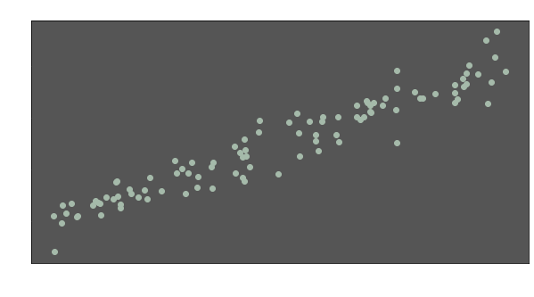
Those data points might express anything. X-axis might represent midterm grades while final grades are denoted by Y-values. Or X and Y values might be expected risk and return metrics of different financial assets respectively. In any case, a model would be useful to understand the data. Thus, we can make inferences about y values when x values are given. We can try to fit a line, like this one:
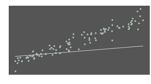
Well, we have a model now (the line). But it does not seem to represent the data well. The slope seems too flat and the line is quite below the many data points. Intuitively, we are aware that the distances between the points and the line have to be shorter.
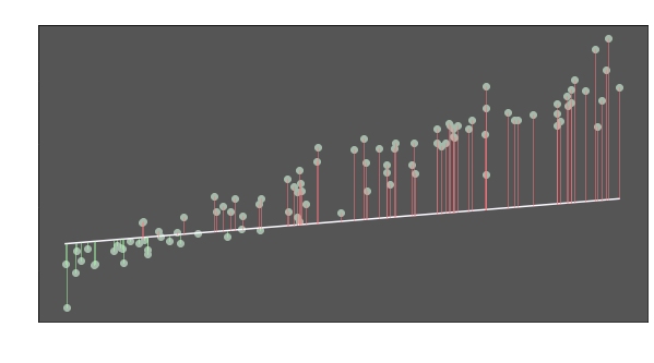
So we want the total of the vertical lines to be as smallest as possible. In other terms, we want to minimize the total of the lengths of the lines. If we call these lines errors, we can formulate them as:
\(e = \hat{y}-y\)
where \(y\) is the actual value of a point and \(\hat{y}\) is its predicted value.
Can we minimize total of those \(e\) values now? Not actually. Our error terms may have positive and negative values. If we sum them up, positive and negative values will cancel each other out. So we need the magnitudes of the errors regardless of their directions.
Here are some alternative ways to measure the magnitude of an error:
- Absolute Error (L1 norm) => \(|\hat{y}-y|\)
- Squared Error (L2 norm) => \((\hat{y}-y)^2\)
- Double Squared Error (L4 norm) => \((\hat{y}-y)^4\)
The common point of all these three is always being non-negative. We can use any of them to find a perfect linear model. If we use L1 norm, we calculate total of absolute differences between \(\hat{y}\) and \(y\). This total is the metric to minimize. We can use mean instead of total since it changes nothing when minimizing the value. We can formulate the metric (Mean Absolute Error) as:
\(MSE = \frac{1}{N}\displaystyle\sum_{k=1}^N|e| =\frac{1}{N}\displaystyle\sum_{k=1}^N|\hat{y}-y| =\frac{1}{N}\displaystyle\sum_{k=1}^N|\beta_ 0+\beta_1x-y|\)
We can also use Mean Squared Error (MSE), which is the most common error function for regression problems:
\(MSE = \frac{1}{N}\displaystyle\sum_{k=1}^Ne^2 =\frac{1}{N}\displaystyle\sum_{k=1}^N(\hat{y}-y)^2 =\frac{1}{N}\displaystyle\sum_{k=1}^N(\beta_ 0+\beta_1x-y)^2\)
The third option is the mean of L4 norms of errors:
\(MDSE = \frac{1}{N}\displaystyle\sum_{k=1}^Ne^4 =\frac{1}{N}\displaystyle\sum_{k=1}^N(\hat{y}-y)^4 =\frac{1}{N}\displaystyle\sum_{k=1}^N(\beta_ 0+\beta_1x-y)^4\)
We will minimize each of them to see the differences. Let’s look at our results:
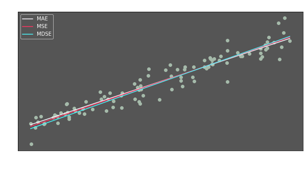
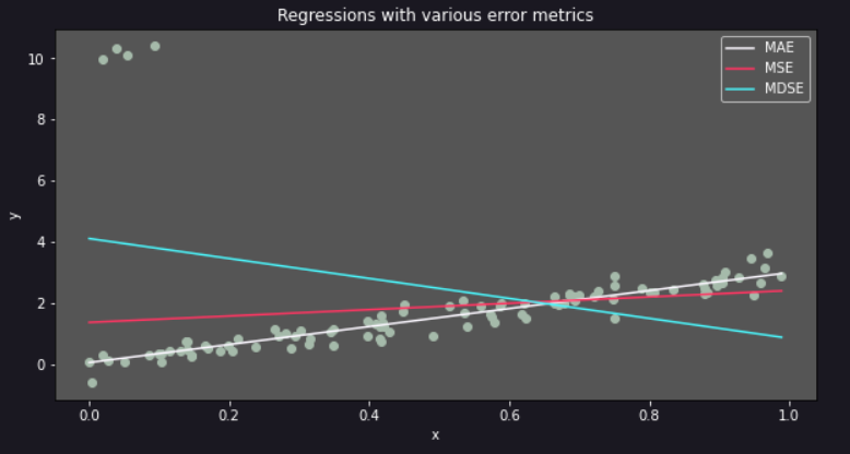
The three regression lines are very similar. It seems like it does not matter which metric is minimized.
But what if the data has OUTLIERS?
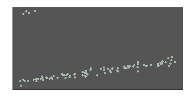
I have multiplied some of the y values with 10. But 96% of our data points are still the same. Let’s calculate the regression lines again:
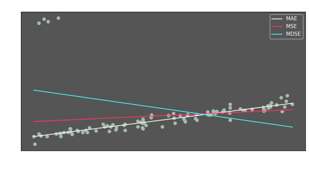
Wow. we have pretty different regression lines. Let’s evaluate them
- MAE
- Outliers did not affect the regression line. They are ignored.
- For 96% of the data, it seems to have best fit.
- MSE
- Outliers have an effect on regression line’s slope.
- MDSE
- Outliers heavily affected the regression line.
- Excluding 4 outlier points, the slope seems meaningless.
So why do we have such different lines after the outliers? The reason is simple. Let’s assume that we have only two error terms: -2 and 3. Total of error norms will be:
- For L1 => TAE = (|-2| + |3|) = 5
- For L2 => TSE = [(-2)² + 3²] = 13
- For L4 => TDSE = [(-2)⁴ + 3⁴] = 97
Let’s look at the share of the second error term (3) in the total error for each norm:
- For TAE => 3/5 = 60%
- For TSE => 9/13 = 69%
- For TDSE => 81/97 = 84%
As you can see, importance of magnitude of an error term is higher for squared and double squared errors. Thus, these regression lines try to get closer to the outliers, which have the highest error terms.
Which of these models is the best? It depends on the situation. In our case, if goal is to get more precise results for most of the observations, then MAE is the best option. However, if high individual errors are unacceptable even if they are rare, MAE does not seem as a good choice. At this point, nonlinear models may also be considered.
