Mean Squared Error
-
-

-
Mean squared error is a frequently used metric to compare model performances. Although its easiness of use is is a sufficient reason to prefer it, another thing makes this metric attractive is its decomposition into meaningful statistical features.
MSE for Estimation
MSE is very handy for comparing the estimators of population or model parameters. Let's deep dive into it.
\(MSE=E\left[ \left( \hat{\theta}-\theta \right)^2 \right]\)
By adding and subtracting \(E[\hat{\theta}]\):
\(MSE=E\left[ \left( \hat{\theta}-\theta+E[\hat{\theta}]-E[\hat{\theta}] \right)^2 \right]\)
We can rearrange the terms:
\(MSE=E\left[ \left( \left( E[\hat{\theta}]-\theta \right)- \left( \hat{\theta}-E[\hat{\theta}] \right) \right)^2 \right]\)
The square expression becomes:
\(MSE=E\left[ \left( E[\hat\theta]-\theta \right)^2 -2\left( E[\hat\theta]-\theta \right)\left( \hat\theta-E[\hat\theta] \right) +\left( \hat\theta-E[\hat\theta] \right)^2 \right]\)
Expectation of sum can be written as sum of expectations:
\(MSE=E\left[ \left( E[\hat\theta]-\theta \right)^2 \right] -2E\left[\left( E[\hat\theta]-\theta \right)\left( \hat\theta-E[\hat\theta] \right)\right] +\left[\left( \hat\theta-E[\hat\theta] \right)^2\right] \)
In here, the first term is the difference between expectation of estimator and the true parameter. It is simply the bias of the estimator. If it is zero, the estimator is unbiased. If it is different than zero, it means that the estimator is not expected to be exactly equal to the parameter.
The third term is simply the variance of the estimator. The second term becomes zero as shown below:
\(MSE=bias^2(\hat\theta,\theta) -2E\left[\left( E[\hat\theta]-\theta \right)\left( \hat\theta-E[\hat\theta] \right)\right] +var(\hat\theta)\)
\(MSE=bias^2(\hat\theta,\theta) -2E\left[ E[\hat\theta]\hat\theta-\left( E[\hat\theta] \right)^2-\theta\hat\theta+E[\hat\theta]\theta \right] +var(\hat\theta)\)
In our formula, The random variable is \(\hat\theta\). The value of true parameter \(\theta\) is constant since it does not affected by the estimator \(\hat\theta\). In addition, \(E\left[E\left[\hat\theta\right]\right] = E\left[\hat\theta\right]\) Since the expectation operator does not affect the expectation of the random variable.
\(MSE=bias^2(\hat\theta,\theta) -2\left( E[\hat\theta] \right)^2 +2\left( E[\hat\theta] \right)^2 +2E[\hat\theta]\theta -2E[\hat\theta]\theta +var(\hat\theta)\)
\(MSE=bias^2(\hat\theta,\theta) +var(\hat\theta)\)
There is a much simpler way to get the same result. We can use the well known variance formula which is \(V\left[ x \right] = E\left[ x^2 \right] - \left( E\left[ x \right] \right)^2\). In other terms: \(E\left[ x^2 \right] = \left( E\left[ x \right] \right)^2+V\left[ x \right]\). Thus:
\(MSE=E\left[ \left( \hat{\theta}-\theta \right)^2 \right]\)
\(MSE= \left(E\left[ \hat{\theta}-\theta \right]\right)^2 + V\left[ \hat{\theta}-\theta \right]\)
In the second term, \(\theta\) is constant. Thus:
\(MSE= \left(E\left[ \hat{\theta}-\theta \right]\right)^2 + V\left[ \hat{\theta} \right]\)
\(MSE=bias^2(\hat\theta,\theta) +var(\hat\theta)\)
MSE for Prediction
It is not only valid for the estimators. Mean squared error of predictions have also a similar decomposition
Let's say true response data has a model such that:
\(y = f(X)+\epsilon\)
And we have a predictive model such as:
\(\hat y = \hat f(X)\)
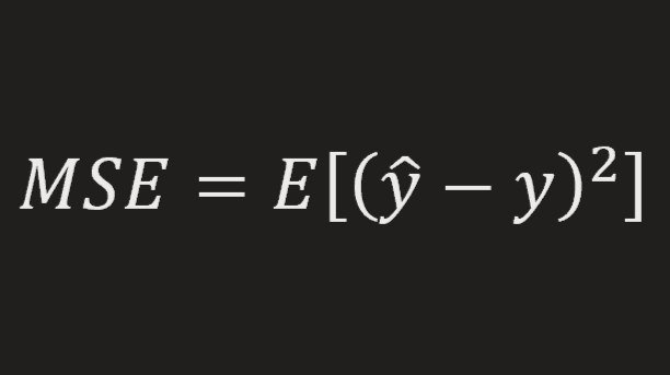
\(MSE=E\left[ \left( \hat{y}-y\right)^2 \right]\)
\(MSE= \left( E\left[ \hat{y}-y \right] \right)^2 +V\left[ \hat{y}-y \right]\)
\(MSE= \left( E\left[ \hat f(X) - f(X)-\epsilon \right] \right)^2 +V\left[ \hat f(X) - f(X)-\epsilon \right]\)
If we can say that \(\hat f(X) - f(X)\) and \(\epsilon\) are uncorrelated:
\(MSE= \left( E\left[ \hat f(X) - f(X)-\epsilon \right] \right)^2 +V\left[ \hat f(X) - f(X) \right] +V\left[ \epsilon \right]\)
\(MSE= bias^2 +variance +irreducible \ error\)
Irreducible error is inevitable due to the randomness in the model. Even if we had the exact model parameters as estimators, we could not aviod the irreducible error.


